5MA+スーパートレンド + Disparity Scalping (SIMPLE FILTER)5MA + ATR Trend Filter + Disparity Scalping
This indicator combines a five-EMA trend framework, an ATR-based trailing trend line, a volatility breakout detector, and an ultra-fast scalping module using RSI and custom momentum prediction.
It is designed for both trend continuation and rapid reversal trading.
🔹 Main Components
1️⃣ Five-EMA Trend Framework
Uses 9 / 20 / 50 / 100 / 200 EMAs
Identifies short-term and long-term market direction
Provides dynamic support and resistance
Helpful for determining breakout vs. pullback conditions
2️⃣ ATR-Based Trailing Trend Line
Uses ATR multiplier to build a trailing stop line
Color change indicates directional shift
Works as a trend filter or trailing stop reference
Helps avoid counter-trend trades during strong trends
3️⃣ High-Volatility Breakout Detector (Optimized for Fast Markets)
Uses ATR expansion, Bollinger band breakout, and volatility comparison (HV vs RV)
Detects sudden market acceleration
Generates breakout BUY/SELL signals when volatility pressure aligns with direction
Useful for explosive markets such as gold or crypto, but compatible with all assets
4️⃣ Ultra-Fast Disparity Scalper
Measures price distance from EMA5 and EMA10
Uses RSI for exhaustion filtering
Predicts momentum turns with a custom RVI-based algorithm
Generates early reversal BUY/SELL signals before full market reaction
Designed for scalping in high-speed environments
5️⃣ Simple Overheat Filter
Blocks trades in extremely overbought/oversold zones
Gray signals indicate low-quality trade setups to avoid
Helps remove “chasing” entries during excessive deviation
🎯 Best Use Cases
Scalping fast reversals
Entering trends after confirmed volatility breakouts
Filtering entries during extreme overbought/oversold phases
Combining EMA structure with breakout momentum
⚠️ Important Notice
This tool is designed to support decision making, not guarantee trade results.
For best performance, combine with:
Price action (market structure)
Volume/volatility context
Support and resistance analysis
🏷️ Short Description (for compact summary)
Five-EMA trend structure with ATR trailing filter, volatility breakout detection, and ultra-fast scalping using RSI + momentum prediction. Suitable for both rapid reversals and trend continuation setups.
Search in scripts for "Trailing stop"

Real Relative Strength Indicator### What is RRS (Real Relative Strength)?
RRS is a volatility-normalized relative strength indicator that shows you – in real time – whether your stock, crypto, or any asset is genuinely beating or lagging the broader market after adjusting for risk and volatility. Unlike the classic “price ÷ SPY” line that gets completely fooled by volatility regimes, RRS answers the only question that actually matters to professional traders:
“Is this ticker moving better (or worse) than the market on a risk-adjusted basis right now?”
It does this by measuring the excess momentum of your ticker versus a benchmark (SPY, QQQ, BTC, etc.) and then dividing that excess by the average volatility (ATR) of both instruments. The result is a clean, centered-around-zero oscillator that works the same way in calm markets, crash markets, or parabolic bull runs.
### How to Use the RRS Indicator (Aqua/Purple Area Version) in Practice
The indicator is deliberately simple to read once you know the rules:
Positive area (aqua) means genuine outperformance.
Negative area (purple) means genuine underperformance.
The farther from zero, the stronger the leadership or weakness.
#### Core Signals and How to Trade Them
- RRS crossing above zero → one of the highest-probability long signals in existence. The asset has just started outperforming the market on a risk-adjusted basis. Enter or add aggressively if price structure agrees.
- RRS crossing below zero → leadership is ending. Tighten stops, take partial or full profits, or flip short if you trade both sides.
- RRS above +2 (bright aqua area) → clear leadership. This is where the real money is made in bull markets. Trail stops, add on pullbacks, let winners run.
- RRS below –2 (bright purple area) → clear distribution or capitulation. Avoid new longs, consider short entries or protective puts.
- Extreme readings above +4 or below –4 (background tint appears) → rare, very high-conviction moves. Treat these like once-a-month opportunities.
- Divergence (not plotted here, but easy to spot visually): price making new highs while the aqua area is shrinking → distribution. Price making new lows while the purple area is shrinking → hidden buying and coming reversal.
#### Best Settings by Style and Asset Class
For stocks and ETFs: keep benchmark as SPY (or QQQ for tech-heavy names) and length 14–20 on daily/4H charts.
For crypto: change the benchmark to BTCUSD (or ETHUSD) immediately — otherwise the reading is meaningless. Length 10–14 works best on 1H–4H crypto charts because volatility is higher.
For day trading: drop length to 10–12 and use 15-minute or 5-minute charts. Signals are faster and still extremely clean.
#### Highest-Edge Setups (What Actually Prints Money)
- RRS crosses above zero while price is still below a major moving average (50 EMA, 200 SMA, etc.) → early leadership, often catches the exact bottom of a new leg up.
- RRS already deep aqua (+3 or higher) and price pulls back to support without RRS dropping below +1 → textbook add-on or re-entry zone.
- RRS deep purple and suddenly turns flat or starts curling up while price is still falling → hidden accumulation, usually the exact low tick.
That’s it. Master these few rules and the RRS becomes one of the most powerful edge tools you will ever use for rotation trading...

Average True Range (ATR)Strategy Name: ATR Trend-Following System with Volatility Filter & Dynamic Risk Management
Short Name: ATR Pro Trend System
Current Version: 2025 Edition (fully tested and optimized)Core ConceptA clean, robust, and highly profitable trend-following strategy that only trades when three strict conditions are met simultaneously:Clear trend direction (price above/below EMA 50)
Confirmed trend strength and trailing stop (SuperTrend)
Sufficient market volatility (current ATR(14) > its 50-period average)
This combination ensures the strategy stays out of choppy, low-volatility ranges and only enters during high-probability, trending moves with real momentum.Key Features & ComponentsComponent
Function
Default Settings
EMA 50
Primary trend filter
50-period exponential
SuperTrend
Dynamic trailing stop + secondary trend confirmation
Period 10, Multiplier 3.0
ATR(14) with RMA
True volatility measurement (Wilder’s original method)
Length 14
50-period SMA of ATR
Volatility filter – only trade when current ATR > average ATR
Length 50
Background coloring
Visual position status: light green = long, light red = short, white = flat
–
Entry markers
Green/red triangles at the exact entry bar
–
Dynamic position sizing
Fixed-fractional risk: exactly 1% of equity per trade
1.00% risk
Stop distance
2.5 × ATR(14) – fully adaptive to current volatility
Multiplier 2.5
Entry RulesLong: Close > EMA 50 AND SuperTrend bullish AND ATR(14) > SMA(ATR,50)
Short: Close < EMA 50 AND SuperTrend bearish AND ATR(14) > SMA(ATR,50)
Exit RulesPosition is closed automatically when SuperTrend flips direction (acts as volatility-adjusted trailing stop).
Money ManagementRisk per trade: exactly 1% of current account equity
Position size is recalculated on every new entry based on current ATR
Automatically scales up in strong trends, scales down in low-volatility regimes
Performance Highlights (2015–Nov 2025, real backtests)CAGR: 22–50% depending on market
Max Drawdown: 18–28%
Profit Factor: 1.89–2.44
Win Rate: 57–62%
Average holding time: 10–25 days (daily timeframe)
Best Markets & TimeframesExcellent on: Bitcoin, S&P 500, Nasdaq-100, DAX, Gold, major Forex pairs
Recommended timeframes: 4H, Daily, Weekly (Daily is the sweet spot)

Adaptive Trend Navigator [ATH Filter & Risk Engine]Description:
This strategy implements a systematic Trend Following approach designed to capture major moves while actively protecting capital during severe bear markets. It combines a classic Moving Average "Fan" logic with two advanced risk management layers: a 4-Stage Dynamic Stop Loss and a macro-economic "Circuit Breaker" filter.
Core Concepts:
1. Trend Identification (Entry Logic) The script uses a cascade of Simple Moving Averages (SMA 25, 50, 100, 200) to identify the maturity of a trend.
Entries are triggered by specific crossovers (e.g., SMA 25 crossing SMA 50) or by breaking above the previous trade's high ("High-Water Mark" Re-Entry).
2. The "Circuit Breaker" (Crash Protection) To prevent trading during historical market collapses (like 2000 or 2008), the strategy monitors the Nasdaq 100 (QQQ) as a global benchmark:
Normal Regime: If the market is within 20% of its All-Time High, the strategy operates normally.
Crisis Regime: If the QQQ falls more than 20% from its ATH, the "Circuit Breaker" activates (Visualized by a Red Background).
Recovery Rule: In a Crisis Regime, new long positions are blocked unless the QQQ reclaims its SMA 200. This filters out "bull traps" in secular bear markets.
3. 4-Stage Risk Engine (Exit Logic) Once in a trade, the risk management adapts to the position's performance:
Stage 1: Fixed initial Stop Loss (default 10%) for breathing room.
Stage 2: Moves to Break-Even area once the price rises 12%.
Stage 3: Tightens to a trailing stop (8%) after 25% profit.
Stage 4: Maximizes gains with a tight trailing stop (5%) during parabolic moves (>40% profit).
Visual Guide:
SMAs: 25/50/100/200 period lines for trend visualization.
Red Background: Indicates the "Crisis Regime" where trading is halted due to broad market weakness.
Blue Background: Indicates a "Recovery Phase" (Crisis is active, but market is above SMA 200).
Red Line: Shows the dynamic Stop Loss level for active positions.
Settings: All parameters (SMA lengths, Drawdown threshold, Risk Stages) are fully customizable. The QQQ benchmark ticker can also be changed to SPY or other indices depending on the asset class traded.

Trend Breakout & Ratchet Stop System [Market Filter]Description:
This strategy implements a robust trend-following system designed to capture momentum moves while strictly managing downside risk through a multi-stage "Ratchet" exit mechanism and broad market filters.
It is designed for swing traders who want to align individual stock entries with the overall market direction.
How it works:
1. Market Regime Filters (The "Safety Check") Before taking any position, the strategy checks the health of the broader market to avoid "catching falling knives."
Broad Market Filter: By default, it checks NASDAQ:QQQ (adjustable). If the benchmark is trading below its SMA 200, the strategy assumes a Bear Market and suppresses all new long entries.
Volatility Filter (VIX): Uses CBOE:VIX to gauge fear. If the VIX is above a specific threshold (Default: 32), entries are paused, and existing positions can optionally be closed to preserve capital.
2. Entry Logic Entries are based on Momentum and Trend confirmation. A position is opened if filters are clear AND one of the following occurs:
Golden Cross: SMA 25 crosses over SMA 50.
SMA Breakouts: A "Three-Bar-Break" logic confirms a breakout above the SMA 50, 100, or 200 (price must establish itself above the moving average).
3. The "Ratchet" Exit System The exit logic evolves as the trade progresses, tightening risk like a ratchet:
Stage 0 (Initial Risk): Starts with a standard percentage Stop Loss from the entry price.
Stage 1 (Breakeven/Lock): Once the price rises by Profit Step 1 (e.g., +10%), the Stop Loss jumps to a tighter level and locks there. This secures the initial move.
Stage 2 (Trailing Mode): If the price continues to rise to Profit Step 2 (e.g., +15%), the Stop Loss converts into a dynamic Trailing Stop relative to the Highest High. This allows the trade to run as long as the trend persists.
Additional Exits:
Dead Cross: Closes position if SMA 25 crosses under SMA 50.
VIX Panic: Emergency exit if volatility spikes above the threshold.
Settings & Customization:
SMAs: Adjustable lengths for all Moving Averages.
Filters: Toggle Market/VIX filters on/off and choose your benchmark ticker (e.g., SPY or QQQ).
Risk Management: Fully customizable percentages for the Ratchet steps (Initial SL, Stage 1 Trigger, Trailing distance).

Bassi's Consolidation Breakout — ULTIMATE PRO + VPOverview
Bassi’s Consolidation Breakout — ULTIMATE PRO + VP is a professional-grade breakout detection system that combines price structure, volume confirmation, volatility compression, and custom volume profile logic.
The indicator automatically detects compressed consolidation zones, confirms breakouts with multi-layer filters, and plots full trade setups including:
Entry level
Stop-loss
TP1, TP2, TP3 (R:R based)
Trend filters + MTF EMA
Retest validation
Volume Profile confirmation (POC / VAH / VAL)
This is one of the most complete breakout frameworks for TradingView.
🔍 Core Concept
The script detects tight consolidation boxes based on:
Price range (% compression)
Lookback period
Minimum required bars
Breakout above/below the box
Once the consolidation ends, breakout signals fire only if they pass all filters.
This focuses your trading on high-probability breakouts only.
🔥 Key Features
1️⃣ Automated Consolidation Box Detection
Draws consolidation boxes dynamically
Identifies tight range compression
Supports advanced range logic for high accuracy
2️⃣ Smart Breakout + Retest Engine
Breakouts and breakdowns require:
Structure break
Minimum breakout expansion (0.15%)
Volume confirmation
Trend (200 EMA) confirmation
Optional retest validation
Optional Volume Profile filter
Each valid breakout prints a signal + full trade setup.
3️⃣ Custom Volume Profile Engine
Fast and lightweight custom-built VP that calculates:
POC (Point of Control)
VAH (Value Area High)
VAL (Value Area Low)
These levels can optionally be used to filter weak breakouts.
4️⃣ Multi-Timeframe Trend Filter
Uses 200 EMA from any selected higher timeframe
Helps avoid counter-trend fakeouts
Fully optional
5️⃣ Automatic Trade Setup Projection
Each breakout generates:
Stop-loss (ATR × multiplier)
TP1 (R:R)
TP2 (R:R)
TP3 (optional)
Clean signal labels
Only keeps the last 2 signals to maintain clarity
6️⃣ Alerts Included
Alerts fire instantly when a valid breakout occurs:
“Bassi LONG + VP”
“Bassi SHORT + VP”
Alerts include ticker + entry price.
📘 Usage Guide & Trading Rules
✔ Recommended Trading Steps
1. Wait for a confirmed consolidation box
Box must be narrow
Must meet minimum bar requirement
2. Wait for a confirmed breakout signal
Signal requires:
Breakout above/below box
Volume confirmation
Trend & MTF confirmation if enabled
Optional retest
Optional VP filter (close outside VAH/VAL)
3. Follow the projected setup
The script prints:
Entry
SL
TP1 / TP2 / TP3
Target lines extend automatically.
📖 How to Use the Script (Trading Rules)
1️⃣ Long Entry Rules
Enter Long when:
Price breaks above trend confirmation level
Momentum signal turns bullish
Candle closes above trigger line
Volatility filter is satisfied
Exit Long:
TP1/TP2/TP3 levels
Reversal signal
Trailing stop hit
2️⃣ Short Entry Rules
Enter Short when:
Price breaks below trend confirmation level
Momentum signal turns bearish
Candle closes below trigger line
Volatility filter is satisfied
Exit Short:
TP1/TP2/TP3 levels
Trend reversal
Trailing stop hit
✔ Recommended Markets
Crypto
Forex
Indices
Futures
Stocks
Works on all timeframes from 1-minute to daily.
✔ Best Practice
Avoid taking signals against HTF trend
Prefer signals that break away from VAH/VAL
Use TP1 to secure partial profits
Move SL to breakeven after TP1 if desired
Always follow personal risk management
👤 Author
Created by: Mahdi Bassi
Professional trader & systems designer
Focused on structural, volume-based and volatility-based strategies.
⚠️ Disclaimer
This script is for educational purposes only.
No indicator can guarantee profits.
Always use proper risk management and trade responsibly.

Float Rotation TrackerFloat Rotation Tracker - Quick Reference Guide
What is Float Rotation?
Float Rotation = Cumulative Daily Volume ÷ Float
Example:
Float = 5,000,000 shares
Day Volume = 7,500,000 shares
Rotation = 7.5M ÷ 5M = 1.5x (150%)
When rotation hits 1x (100%), every available share has theoretically changed hands at least once during the trading day.
Why It Matters
RotationMeaningImplication0.5x50% of float tradedInterest building1.0x 🔥Full rotationExtreme interest confirmed2.0x 🔥🔥Double rotationVery high volatility3.0x 🔥🔥🔥Triple rotationRare - maximum volatility
Key insight: High rotation on a low-float stock = explosive potential
Float Classification
Float SizeClassificationRotation Impact≤ 2M🔥 MICROExtremely volatile, fast rotation≤ 5M🔥 VERY LOWExcellent momentum potential≤ 10MLOWGood for rotation plays> 10MNORMALNeeds massive volume to rotate
Rule of thumb: Focus on stocks with float under 10M for meaningful rotation signals.
Reading the Indicator
Rotation Line (Yellow)
Shows current rotation level
Rises throughout the day as volume accumulates
Crosses horizontal level lines at milestones
Level Lines
LineColorMeaning0.5Gray dotted50% rotation1.0Orange solidFull rotation2.0Red solidDouble rotation3.0Fuchsia solidTriple rotation
Volume Bars (Bottom)
ColorMeaningGrayBelow average volumeBlueNormal volume (1-2x avg)GreenHigh volume (2-5x avg)LimeExtreme volume (5x+ avg)
Milestone Markers
Circles appear when rotation crosses key levels
Labels show "50%", "1x", "2x", "3x🔥"
Background Color
Changes as rotation increases
Darker = higher rotation level
Info Table Explained
FieldDescriptionFloatShare count + classification (MICRO/LOW/NORMAL)SourceAuto ✓ = TradingView data / Manual = user enteredRotationCurrent rotation with emoji indicatorRotation %Same as rotation × 100Day VolumeCumulative volume todayTo XxVolume needed to reach next milestoneBar RVolCurrent bar's relative volumeMilestonesWhich levels have been hit todayPer RotationShares equal to one full rotationEst. TimeBars until next milestone (at current pace)
Trading with Float Rotation
Entry Signals
Early Entry (Higher Risk, Higher Reward)
Rotation approaching 0.5x
Strong price action (bull flag, breakout)
Rising relative volume bars
Confirmation Entry (Lower Risk)
Rotation at or above 1x
Price holding above VWAP
Continuous green/lime volume bars
Late Entry (Highest Risk)
Rotation above 2x
Only enter on clear pullback pattern
Tight stop required
Exit Signals
Warning Signs:
Rotation very high (2x+) with declining volume bars
Reversal candle after milestone
Price breaking below key support
Volume bars turning gray/blue after being green/lime
Take Profits:
Partial profit at each rotation milestone
Trail stop as rotation increases
Full exit on reversal pattern after 2x+ rotation
Best Setups
Ideal Float Rotation Play
✓ Float under 10M (preferably under 5M)
✓ Stock up 5%+ on the day
✓ News catalyst driving interest
✓ Rotation approaching or exceeding 1x
✓ Price above VWAP
✓ Volume bars green or lime
✓ Clear chart pattern (bull flag, flat top)
Red Flags to Avoid
✗ Float over 50M (hard to rotate meaningfully)
✗ Rotation high but price declining
✗ Volume bars turning gray after spike
✗ No clear catalyst
✗ Price below VWAP with high rotation
✗ Late in day (3pm+) after 2x rotation
Float Data Sources
If auto-detect doesn't work, get float from:
SourceHow to FindFinvizfinviz.com → ticker → "Shs Float"Yahoo FinanceFinance.yahoo.com → Statistics → "Float"MarketWatchMarketwatch.com → ticker → ProfileYour BrokerUsually in stock details/fundamentals
Note: Float can change due to offerings, buybacks, lockup expirations. Check recent data.
Settings Guide
Conservative Settings
Alert Level 1: 0.75 (75%)
Alert Level 2: 1.0 (100%)
Alert Level 3: 2.0 (200%)
Alert Level 4: 3.0 (300%)
High Vol Multiplier: 2.0
Extreme Vol Multiplier: 5.0
Aggressive Settings
Alert Level 1: 0.3 (30%)
Alert Level 2: 0.5 (50%)
Alert Level 3: 1.0 (100%)
Alert Level 4: 2.0 (200%)
High Vol Multiplier: 1.5
Extreme Vol Multiplier: 3.0
Alert Setup
Recommended Alerts
100% Rotation (1x) - Primary signal
Most important milestone
Confirms extreme interest
High Rotation + Extreme Volume
Combined condition
Very high probability signal
How to Set
Right-click chart → Add Alert
Condition: Float Rotation Tracker
Select desired milestone
Set notification (popup/email/phone)
Set expiration
Common Questions
Q: Why is my float showing "Manual (no data)"?
A: TradingView doesn't have float data for this stock. Enter the float manually in settings after looking it up on Finviz or Yahoo Finance.
Q: The rotation seems too high/low - is the float wrong?
A: Possibly. Cross-check float on Finviz. Recent offerings or share structure changes may not be reflected in TradingView's data.
Q: What if float rotates early in the day?
A: Early 1x rotation (within first hour) is very bullish - indicates massive interest. Watch for continuation patterns.
Q: High rotation but price is dropping?
A: This is distribution - large holders are selling into demand. High rotation doesn't guarantee price direction, just volatility.
Q: Can I use this for swing trading?
A: The indicator resets daily, so it's designed for intraday use. You could note multi-day rotation patterns manually.
Quick Decision Matrix
RotationPrice ActionVolumeDecision<0.5xStrong upHighWatch, early stage0.5-1xConsolidatingSteadyPrepare entry1x+Breaking outIncreasingEntry on pattern1x+DroppingHighAvoid - distribution2x+Strong upExtremePartial profit, trail stop2x+Reversal candleDecliningExit or avoid
Workflow Integration
MORNING ROUTINE:
1. Scan for gappers (5%+, high volume)
2. Check float on each candidate
3. Apply Float Rotation Tracker
4. Prioritize lowest float with building rotation
DURING SESSION:
5. Watch rotation levels on active trades
6. Enter on patterns when rotation confirms (0.5-1x)
7. Scale out as rotation increases
8. Exit or trail after 2x rotation
END OF DAY:
9. Note which stocks hit 2x+ rotation
10. Review rotation vs price action
11. Learn patterns for future trades
Combining with Other Indicators
IndicatorHow to Use Together5 PillarsScreen for low-float stocks firstGap & GoCheck rotation on gappersBull FlagEnter bull flags with 1x+ rotationVWAPOnly trade rotation plays above VWAPRSIWatch for divergence at high rotation
Key Takeaways
Float size matters - Lower float = faster rotation = more volatility
1x is the key level - Full rotation confirms extreme interest
Volume quality matters - Green/lime bars better than gray
Combine with price action - Rotation confirms, patterns trigger
Know when you're late - 2x+ rotation is late stage
Check your float data - Wrong float = wrong rotation calculation
Happy Trading! 🔥

Fractional Candlestick Long Only Experimental V10Fractional Candlestick Long-Only Strategy – Technical Description
This document provides a professional English description of the "Fractional Candlestick Long Only Experimental V6" strategy using pure CF/AB fractional kernels and wavelet-based filtering.
1. Fractional Candlesticks (CF / AB)
The strategy computes two fractional representations of price using Caputo–Fabrizio (CF) and Atangana–Baleanu (AB) kernels. These provide long-memory filtering without EMA approximations. Both CF and AB versions are applied to O/H/L/C, producing fractional candlesticks and fractional Heikin-Ashi variants.
2. Trend Stack Logic
Trend confirmation is based on a 4-component stack:
- CF close > AB close
- HA_CF close > HA_AB close
- HA_CF bullish
- HA_AB bullish
The user selects how many components must align (4, 3, or any 2).
3. Wavelet Filtering
A wavelet transform (Haar, Daubechies-4, Mexican Hat) is applied to a chosen source (e.g., HA_CF close). The wavelet response is used as:
- entry filter (4 modes)
- exit filter (4 modes)
Wavelet modes: off, confirm, wavelet-only, block adverse signals.
4. Trailing System
Trailing stop uses fractional AB low × buffer, providing long-memory dynamic trailing behavior. A fractional trend channel (CF/AB lows vs HA highs) is also plotted.
5. Exit Framework
Exit options include: stack flip, CF

SuperTrend Dual RMAOverview
The SuperTrend Dual RMA is a hybrid volatility-based trend-following system that merges two Relative Moving Averages (RMAs) with an Average True Range (ATR)–anchored SuperTrend framework. The primary purpose of this indicator is to offer a smoother and more reliable depiction of directional bias while maintaining sensitivity to price volatility and market volume.
Traditional SuperTrend implementations typically rely on a single moving average and a fixed volatility envelope. This dual RMA structure introduces an adaptive central tendency line that reacts proportionally to both price and volume, allowing for more nuanced identification of trend reversals and continuation patterns.
**Core Concept**
The indicator is built around two key principles — smoothing and volatility adaptation.
1. **Smoothing:** The use of two separate RMAs with configurable lengths creates a dynamic equilibrium between short-term responsiveness and long-term stability. The first RMA captures near-term directional shifts, while the second provides broader market context. The average of both becomes the foundation of the SuperTrend bands.
2. **Volatility Adaptation:** The ATR multiplier and period define the distance between upper and lower bands relative to recent volatility. This ensures that the SuperTrend line remains flexible across varying market conditions — expanding during high volatility and contracting during calm phases.
**Calculation Steps**
* The indicator first computes two volume-weighted RMAs based on the typical price (`hlc3`) multiplied by trading volume.
* Each RMA is normalized by the smoothed volume to maintain proportional weighting.
* These two RMAs are averaged to produce a “basis line” that reflects the current market consensus price.
* The ATR is calculated over a user-defined period, then multiplied by a volatility factor (ATR multiplier).
* The resulting ATR value defines dynamic upper and lower thresholds around the basis line.
* Trend direction is determined by price closing behavior relative to these thresholds:
* When the closing price exceeds the upper band, the trend is considered bullish.
* When it drops below the lower band, the trend turns bearish.
* If price remains within the bands, the prior trend direction is maintained for consistency.
**Visual Structure**
The SuperTrend Dual RMA provides multiple layers of visual feedback for enhanced interpretation:
* Two distinct RMA lines (short and long) are plotted with complementary colors for contrast and clarity.
* A soft fill between the RMA lines highlights the interaction between short- and medium-term momentum.
* The ATR-based SuperTrend bands are drawn above and below the basis, with adaptive coloring that corresponds to the prevailing trend direction.
* Bar colors automatically adjust to reflect bullish or bearish bias, making it easy to identify trend shifts without relying solely on crossovers.
* Optional triangle markers appear below or above bars to signal potential buy or sell opportunities based on crossover logic.
**Signals and Alerts**
The indicator provides real-time crossover detection:
* **Buy Signal:** Triggered when the closing price moves above the SuperTrend line, confirming potential bullish continuation or reversal.
* **Sell Signal:** Triggered when the closing price drops below the SuperTrend line, indicating possible bearish momentum or reversal.
Both conditions have built-in `alertcondition()` functions, allowing users to set automated alerts for trading or monitoring purposes. This enables integration with TradingView’s alert system for push notifications, emails, or webhook connections.
**Usage Guidelines**
* **Trend Identification:** Use the color-coded trend line and bar color as a visual guide to the current directional bias.
* **Entry and Exit Timing:** Consider entering trades when a new crossover alert appears, preferably in the direction of the overall higher-timeframe trend.
* **Parameter Tuning:** Adjust the RMA lengths and ATR parameters based on asset volatility. Shorter RMA and ATR settings provide faster reactions, suitable for intraday or high-frequency trading, while longer configurations better fit swing or position strategies.
* **Risk Management:** Because the SuperTrend inherently acts as a dynamic stop level, traders can use the opposite band or SuperTrend line as a trailing stop or exit signal.
**Practical Applications**
* Trend confirmation in multi-timeframe strategies.
* Adaptive trailing stop placement using the lower or upper band.
* Visual comparison of volume-weighted price movement against volatility envelopes.
* Integration into algorithmic trading systems as a signal filter or trend bias component.
* Identification of overextended conditions when price significantly diverges from the SuperTrend basis.
**Originality and Advantages**
The SuperTrend Dual RMA differentiates itself from conventional SuperTrend scripts through three innovative design choices:
1. **Dual Volume-Weighted RMAs:** By incorporating two RMAs weighted by trading volume, the indicator accounts for liquidity dynamics, producing smoother and more reliable averages compared to price-only calculations.
2. **Anchored SuperTrend Framework:** The SuperTrend bands are not derived from a fixed source (such as a single close or median price) but from a blended RMA basis, making them more adaptable to varying market behaviors.
3. **Integrated Multi-Layer Visualization:** The inclusion of filled regions between RMAs, dynamic band coloring, and bar tinting enhances readability and analytical depth without overwhelming the chart.
These improvements collectively create a more balanced and data-rich representation of market structure, offering a higher degree of analytical precision. It’s suitable for traders seeking both discretionary and systematic use, as the indicator’s logic is transparent and compatible with alert-based or automated workflows.
**Summary**
The SuperTrend Dual RMA is a refined evolution of the classic SuperTrend, optimized for traders who value smoother directional tracking and more intelligent volatility adaptation. It blends two time-sensitive, volume-aware moving averages with an ATR-derived volatility system to deliver reliable, actionable trend information. Its visual design, adaptive responsiveness, and integrated alert functionality make it a complete solution for identifying and managing trends across multiple asset classes and timeframes.

ATM Pulse (Arjo)ATM Pulse (Arjo) — Real-Time ATM Options Sentiment & Trend Strength Indicator
Overview
ATM Pulse (Arjo) is an options analytics and trend overlay tool that automatically detects the At-The-Money (ATM) strike for NIFTY, BANKNIFTY , or any selected stock.
It merges Call–Put Volume Ratio (CPVR) sentiment analysis with a Chandelier Exit trend overlay to help traders visualize both market bias and trend direction in a single chart.
Concepts & Logic
ATM Auto Detection
The script calculates the current ATM strike by rounding the underlying’s price to the nearest strike interval (e.g., 50 for NIFTY, 100 for BANKNIFTY). It then requests live option-chain data for that strike.
Call–Put Volume Ratio (CPVR)
The Call-Put Volume Ratio (CPVR) is calculated as the call volume divided by the put volume.
CPVR > 1.25 → Bullish dominance (Calls stronger)
CPVR < 0.75 → Bearish dominance (Puts stronger)
0.75–1.25 → Neutral sentiment
This ratio helps interpret real-time option-market positioning.
Chandelier Exit Trend Overlay
Using Average True Range (ATR) , the overlay plots dynamic trailing stops and visual trend zones:
🟢 Green: Uptrend continuation zone
🔴 Red: Downtrend continuation zone
A color change signals possible momentum reversal.
Combination of CPVR and Chandelier Exit
CPVR gauges option-market sentiment
Chandelier Exit confirms price-action direction
When both align (e.g., bullish CPVR + green Chandelier zone), it strengthens directional conviction. Divergent readings may signal indecision or early reversals.
How to Use
Open any NIFTY, BANKNIFTY , or stocks chart.
Add ATM Pulse (Arjo) to the chart.
Select your expiry date — the script auto-detects the ATM strike and displays:
C: Call LTP
P: Put LTP
CPVR: Call/Put Volume Ratio label
Watch the Chandelier Exit colors:
🟢 Green = Bullish trend
🔴 Red = Bearish trend
Combine CPVR bias + trend color for confirmation.
If CPVR is above 1.25 and trend color green → More bullish activity (Calls stronger).
If CPVR is below 0.75, and trend color red→ More bearish activity (Puts stronger).
If CPVR is between 0.75 and 1.25 and the trend color is gray/mixed → Neutral
Practical Use Case
The script continuously updates the ATM strike, CPVR , and trend overlay in real time.
It provides a clear visual snapshot of how option volumes align with price momentum , ideal for intraday or short-term directional traders.
Disclaimer
This tool is for educational and analytical purposes only.
It does not provide financial advice or guaranteed trading signals.
Happy Trading. ARJO

AMF PG Strategy v2.3AMF PG Strategy v2.3
1. Core Philosophy: Filtered and Volatility-Aware Trend Following
"AMF PG Strategy" is an advanced trend-following system designed to adapt to the dynamic nature of modern markets. The strategy's core philosophy is not just to follow the trend but also to wait for the right conditions to enter the market.
This is not a "black box." It is a rules-based framework that gives the user full control over various market filters. By requiring multiple conditions to be met simultaneously, the strategy aims to filter out low-quality signals and focus only on high-probability trend opportunities.
2. Core Engine: AMF PG Trend Following
At the heart of the strategy is a proprietary, volatility-aware trend-following mechanism called AMF PG (Praetorian Guard). This engine operates as follows:
Dynamic Bands: Creates a dynamic upper and lower band around the price that is constantly recalculated. The width of these bands is not fixed; It dynamically adjusts based on recent market volatility, volume flow, and price expansion. This adaptive structure allows the strategy to adapt to both calm and high-volatility markets.
Entry Signals: A buy signal is triggered when the price rises above the upper band. A sell signal is triggered when the price falls below the lower band. However, these signals are executed only when all the active filters described below give the green light.
Trailing Stop-Loss: When a position is entered, the opposite band automatically acts as a trailing stop-loss level. For example, when a buy position is opened, the lower band follows the price as a stop-loss. This allows for profit retention and trend continuation.
3. Multi-Layered Filter System: Understanding the Market
The power of this strategy comes from its modular filter system, which allows the user to filter market conditions based on their own analysis. Each filter can be enabled or disabled individually in the settings:
Filter 1: Trend Strength (ADX Filter): This filter confirms whether there is a strong trend in the market. It uses the ADX (Average Directional Index) indicator and only allows trades if the ADX value is above a certain threshold. This helps avoid trading in weak or directionless markets. It also confirms the direction of the trend by checking the position of the DMI (+DI and -DI) lines.
Filter 2: Sideways Market (Chop Index Filter): This filter determines whether the market is excessively choppy or directionless. Using the Chop Index, this filter aims to protect against fakeouts by blocking trades when the market is highly indecisive.
Filter 3: Market Structure (Hurst Exponent Filter): This is one of the strategy's most advanced filters. It analyzes the current market behavior using the Hurst Exponent. This mathematical tool attempts to determine whether a market tends to trend (permanent), tends to revert to the mean (anti-permanent), or moves randomly. This filter ensures that signals are generated only when market structure supports trending trades.
4. Risk Management: Maximum Drawdown Protection
This strategy includes a built-in capital protection mechanism. Users can specify the percentage of their capital they will tolerate to decline from its peak. If the strategy's capital reaches this set drawdown limit, the protection feature is activated, closing all open positions and preventing new trades from being opened. This acts as an emergency brake to protect capital against unexpected market conditions.
5. Automation Ready: Customizable Webhook Alerts
The strategy is designed for traders who want to automate their signals. From the Settings menu, you can configure custom alert messages in JSON format, compatible with third-party automation services (via Webhooks).
6. Strategy Backtest Information
Please note that past performance is not indicative of future results. The published chart and performance report were generated on the 4-hour timeframe of the BTCUSD pair with the following settings:
Test Period: January 1, 2016 - October 31, 2025
Default Position Size: 15% of Capital
Pyramiding: Closed
Commission: 0.0008
Slippage: 2 ticks (Please enter the slippage you used in your own tests)
Testing Approach: The published test includes 423 trades and is statistically significant. It is strongly recommended that you test on different assets and timeframes for your own analysis. The default settings are a template and should be adjusted by the user for their own analysis.

VWAP & Band Cross Strategy v6 - AdvancedThese are a few updates made to the original script. The daily take profit and stop loss functions correctly for 1 contract but because of the pyramiding input even if not used you'll need to multiply the values by the number of contracts to keep consistent results. I have been unable to correct that function. Let me know if you test the script and have any recommendations for improvement. If trading an actual account I do recommend setting hard daily limits with your provider because there is still slippage from the original exit alerts even with the daily stop loss in place.
1. Real-Time Execution & Hard PnL Limits (The Focus)
The most critical changes were implemented to ensure the daily profit and loss limits act as hard, real-time barriers instead of waiting for the candle to close.
• Intrabar Tick Execution: The parameter calc_on_every_tick=true was added to the strategy() declaration. This forces the entire script to re-evaluate its logic on every single price update (tick), enabling immediate action.
• Real-Time PnL Tracking: The PnL calculation was updated to track the total_daily_pnl by summing the realized profit/loss (from closed trades) and the unrealized profit/loss (strategy.openprofit) on every tick.
• Immediate Closure: The script now checks the total_daily_pnl against the user-defined limits (daily_take_profit_value, daily_stop_loss_value) and immediately executes strategy.close_all() the moment the threshold is breached, preventing further trading.
• Combined Risk Enforcement: The user-defined "Max Intraday Risk ($)" and the "Daily Stop Loss (Value)" are compared, and the script enforces the tighter of the two limits.
2. Visibility and External Alerting
To address the unavoidable issue of slippage (which causes price overshoot in fast markets even with tick execution), dedicated alert mechanisms were added.
• Dedicated Alert Condition: An alertcondition named DAILY PNL LIMIT REACHED was added. This allows you to set up a TradingView alert that triggers the instant the daily_limit_reached variable turns true, giving you the fastest possible notification.
• Visual Marker: A large red triangle (\u25b2) is plotted on the chart using plotchar at the exact moment the daily limit condition is met, providing a clear visual confirmation of the trigger bar.
3. Strategy Features and Input Flexibility
Several user-requested features were integrated to make the strategy more robust and customizable.
• Trailing Stop / Breakeven (TSL/BE): A new exit option, Fixed Ticks + TSL, was added, allowing you to set a fixed profit target while also deploying a trailing stop or breakeven level based on points/ticks gained.
• Multiple Exit Types: The exit strategy was expanded to include logic for several types: Fixed Ticks, ATR-based, Capped ATR-based, VWAP Cross, and Price/Band Crosses.
• Pyramiding Control: An input Max Pyramiding Entries was introduced to control how many positions the strategy can have open at the same time.
• Confirmation Logic Toggle: Added an input to choose how multiple confirmation indicators (RSI, SMMA, MACD) are combined: "AND" (all must be true) or "OR" (at least one must be true).
• Indicator Confirmations: Logic for three external indicators—RSI, SMMA (EMA), and MACD—was fully integrated to act as optional filters for entry.
• VWAP Reset Anchors: Logic was corrected to properly reset the VWAP calculation based on the selected period ("Daily", "Weekly", or "Session") by using Pine Script v6's required anchor series.
Trading Day Filters: Inputs were added to select which specific days of the week the strategy is allowed to trade.

Enhanced OB Retest Strategy v7.0The OB Retest Strategy is a full Order Block retest trading system that detects, plots, and trades OB zones across multiple timeframes. It uses structure breaks, retrace depth, and ATR filters to identify strong reversal or continuation setups.
⸻
⚙️ Core Features
• Multi-timeframe OB detection using break-of-structure (BOS) logic
• Automatic zone creation for bullish and bearish order blocks
• Smart merging of overlapping OB zones
• Dynamic flip-zone logic that turns invalidated OBs into new zones
• Wick zone detection for high-precision entries
• ATR-based trailing stop and optional breakeven
• Adjustable retrace depth, breakout %, and ATR filters
• Built-in performance table showing PnL, win rate, and total trades
• Fully backtestable with date range and commission control
⸻
🧠 Logic Summary
1. Detects a BOS on the higher timeframe.
2. Identifies the last opposing candle as the valid OB.
3. Validates the OB based on ATR size and breakout strength.
4. Waits for price to retest the zone to a set depth.
5. Executes trades and manages exits using trailing stop or breakeven.
6. Flips invalidated zones automatically.
⸻
💡 Usage Tips
• Best used on 1H to 4H charts for swing setups.
• Tune ATR and breakout thresholds for your market’s volatility.
• Combine with higher-timeframe bias or liquidity levels for better accuracy.
⸻
⚠️ Notes
• For educational and testing purposes only.
• Backtested results do not predict future performance.
• Always test before live use.

UTBotLibrary "UTBot"
is a powerful and flexible trading toolkit implemented in Pine Script. Based on the widely recognized UT Bot strategy originally developed by Yo_adriiiiaan with important enhancements by HPotter, this library provides users with customizable functions for dynamic trailing stop calculations using ATR (Average True Range), trend detection, and signal generation. It enables developers and traders to seamlessly integrate UT Bot logic into their own indicators and strategies without duplicating code.
Key features include:
Accurate ATR-based trailing stop and reversal detection
Multi-timeframe support for enhanced signal reliability
Clean and efficient API for easy integration and customization
Detailed documentation and examples for quick adoption
Open-source and community-friendly, encouraging collaboration and improvements
We sincerely thank Yo_adriiiiaan for the original UT Bot concept and HPotter for valuable improvements that have made this strategy even more robust. This library aims to honor their work by making the UT Bot methodology accessible to Pine Script developers worldwide.
This library is designed for Pine Script programmers looking to leverage the proven UT Bot methodology to build robust trading systems with minimal effort and maximum maintainability.
UTBot(h, l, c, multi, leng)
Parameters:
h (float) - high
l (float) - low
c (float)-close
multi (float)- multi for ATR
leng (int)-length for ATR
Returns:
xATRTS - ATR Based TrailingStop Value
pos - pos==1, long position, pos==-1, shot position
signal - 0 no signal, 1 buy, -1 sell

Mayer Mutiple | QRMayer Multiple | QR — Publication Description
What it does
Mayer Multiple | QR is a cycle/valuation style oscillator that measures how far price sits above or below its longer-term average and normalizes that distance by current volatility. It helps you spot overheated extensions and deep discounts relative to trend, with adaptive bands that expand/contract as conditions change.
How it works (principle)
The script compares price to a long lookback moving average (default uses a 200-period average of ohlc4) and turns that gap into an oscillator.
It then computes a rolling standard deviation of that oscillator to build dynamic upper/lower bands (±1σ, ±2σ, ±3σ).
When the oscillator rises above the upper bands, the move is statistically stretched (potential distribution/risk). When it falls below the lower bands, it’s statistically depressed (potential accumulation/opportunity).
A small baseline band around zero (scaled from volatility) provides a quick trend-bias read without crowding the view.
Why this matters: Classic “Mayer Multiple” tools use a fixed threshold over a single moving average. This version is volatility-aware: its bands adapt to the market’s current dispersion, reducing false signals in quiet regimes and avoiding constant “overheat” flags in high-vol regimes.
What you see on the chart
White oscillator line: volatility-normalized deviation from the long-term average.
Adaptive bands:
Upper 1/2/3σ (shaded blue tones) = progressively more extended.
Lower 1/2/3σ (shaded green tones) = progressively more discounted.
Baseline ribbon: subtle band around zero for quick bias.
Background highlights: optional flashes when the oscillator exceeds the ±3σ extremes.
All visuals are generated by this script alone; no other indicator is required to understand usage.
How to use it
Context: Use on higher timeframes to gauge where price sits versus its long-term “fair value corridor.”
Signal reading:
Above +1σ/+2σ/+3σ: extension → consider de-risking, trailing stops, or waiting for mean reversion.
Below −1σ/−2σ/−3σ: discount → consider scaling in, watching for trend resumption cues.
Confluence: Treat it as a condition, not a trigger. Pair with structure (higher highs/lows), breadth, or momentum for entries/exits.
Regime awareness: As volatility rises, bands widen; prioritize trend context over single print extremes.
Inputs you can tune
Color mode: preset palettes for lines/fills/backgrounds.
Dynamic Threshold Length: lookback for the volatility (σ) calculation driving the adaptive bands.
Source: price input used for the long-term reference.
Band toggles: show/hide ±1σ / ±2σ / ±3σ envelopes to reduce clutter.
Originality & value
Adaptive, volatility-aware implementation of a Mayer-style concept: rather than one fixed threshold, it scales to current regime, keeping readings comparable across cycles.
Clear, clean presentation (oscillator + bands + optional background) designed for publication with a clean chart so the script’s output is immediately identifiable.
Offers actionable context (stretch/discount zones) while leaving trade execution to the user’s process.
Limitations & good practices
Best used for context and risk framing, not stand-alone entries.
Adaptive bands depend on the lookback you choose; very short windows can overfit, very long windows can lag.
Extremes can persist in strong trends—don’t fade momentum blindly.
Disclaimer
This tool is for research and education only and not investment advice. Markets involve risk. Past performance does not predict or guarantee future results. Use prudent risk management and test settings on your instruments/timeframes.

Trend Magic EMA RMI Trend Sniper📌 Indicator Name:
Trend Magic + EMA + MA Smoothing + RMI Trend Sniper
📝 Description:
This is a multi-functional trend and momentum indicator that combines four powerful tools into a single overlay:
Trend Magic – Plots a dynamic support/resistance line based on CCI and ATR.
Helps identify trend direction (green = bullish, red = bearish).
Acts as a trailing stop or dynamic level for trade entries/exits.
Exponential Moving Average (EMA) – Smooths price data to highlight the underlying trend.
Customizable length, source, and offset.
Serves as a trend filter or moving support/resistance.
MA Smoothing + Bollinger Bands (Optional) – Adds a secondary smoothing filter based on your choice of SMA, EMA, WMA, VWMA, or SMMA.
Optional Bollinger Bands visualize volatility expansion/contraction.
Great for spotting consolidations and breakout opportunities.
RMI Trend Sniper – A momentum-based system combining RSI and MFI.
Highlights bullish (green) or bearish (red) conditions.
Plots a Range-Weighted Moving Average (RWMA) channel to gauge price positioning.
Provides visual BUY/SELL labels and optional bar coloring for fast decision-making.
📊 Uses & Trading Applications:
✅ Trend Identification: Spot the dominant market direction quickly with Trend Magic & EMA.
✅ Momentum Confirmation: RMI Sniper helps confirm whether the market has strong bullish or bearish pressure.
✅ Dynamic Support/Resistance: Trend Magic & EMA act as adaptive levels for stop-loss or trailing positions.
✅ Volatility Analysis: Optional Bollinger Bands show squeezes and potential breakout setups.
✅ Entry/Exit Signals: BUY/SELL alerts and color-coded candles make spotting trade opportunities simple.
💡 Best Use Cases:
Swing Trading: Follow Trend Magic + EMA alignment for higher probability trades.
Scalping/Intraday: Use RMI signals with bar coloring for quick momentum entries.
Trend Following Strategies: Ride trends until Trend Magic flips direction.
Breakout Trading: Watch for price closing outside the Bollinger Bands with RMI confirmation.

Deadband Hysteresis Filter [BackQuant]Deadband Hysteresis Filter
What this is
This tool builds a “debounced” price baseline that ignores small fluctuations and only reacts when price meaningfully departs from its recent path. It uses a deadband to define how much deviation matters and a hysteresis scheme to avoid rapid flip-flops around the decision boundary. The baseline’s slope provides a simple trend cue, used to color candles and to trigger up and down alerts.
Why deadband and hysteresis help
They filter micro noise so the baseline does not react to every tiny tick.
They stabilize state changes. Hysteresis means the rule to start moving is stricter than the rule to keep holding, which reduces whipsaw.
They produce a stepped, readable path that advances during sustained moves and stays flat during chop.
How it works (conceptual)
At each bar the script maintains a running baseline dbhf and compares it to the input price p .
Compute a base threshold baseTau using the selected mode (ATR, Percent, Ticks, or Points).
Build an enter band tauEnter = baseTau × Enter Mult and an exit band tauExit = baseTau × Exit Mult where typically Exit Mult < Enter Mult .
Let diff = p − dbhf .
If diff > +tauEnter , raise the baseline by response × (diff − tauEnter) .
If diff < −tauEnter , lower the baseline by response × (diff + tauEnter) .
Otherwise, hold the prior value.
Trend state is derived from slope: dbhf > dbhf → up trend, dbhf < dbhf → down trend.
Inputs and what they control
Threshold mode
ATR — baseTau = ATR(atrLen) × atrMult . Adapts to volatility. Useful when regimes change.
Percent — baseTau = |price| × pctThresh% . Scale-free across symbols of different prices.
Ticks — baseTau = syminfo.mintick × tickThresh . Good for futures where tick size matters.
Points — baseTau = ptsThresh . Fixed distance in price units.
Band multipliers and response
Enter Mult — outer band. Price must travel at least this far from the baseline before an update occurs. Larger values reject more noise but increase lag.
Exit Mult — inner band for hysteresis. Keep this smaller than Enter Mult to create a hold zone that resists small re-entries.
Response — step size when outside the enter band. Higher response tracks faster; lower response is smoother.
UI settings
Show Filtered Price — plots the baseline on price.
Paint candles — colors bars by the filtered slope using your long/short colors.
How it can be used
Trend qualifier — take entries only in the direction of the baseline slope and skip trades against it.
Debounced crossovers — use the baseline as a stabilized surrogate for price in moving-average or channel crossover rules.
Trailing logic — trail stops a small distance beyond the baseline so small pullbacks do not eject the trade.
Session aware filtering — widen Enter Mult or switch to ATR mode for volatile sessions; tighten in quiet sessions.
Parameter interactions and tuning
Enter Mult vs Response — both govern sensitivity. If you see too many flips, increase Enter Mult or reduce Response. If turns feel late, do the opposite.
Exit Mult — widening the gap between Enter and Exit expands the hold zone and reduces oscillation around the threshold.
Mode choice — ATR adapts automatically; Percent keeps behavior consistent across instruments; Ticks or Points are useful when you think in fixed increments.
Timeframe coupling — on higher timeframes you can often lower Enter Mult or raise Response because raw noise is already reduced.
Concrete starter recipes
General purpose — ATR mode, atrLen=14 , atrMult=1.0–1.5 , Enter=1.0 , Exit=0.5 , Response=0.20 . Balanced noise rejection and lag.
Choppy range filter — ATR mode, increase atrMult to 2.0, keep Response≈0.15 . Stronger suppression of micro-moves.
Fast intraday — Percent mode, pctThresh=0.1–0.3 , Enter=1.0 , Exit=0.4–0.6 , Response=0.30–0.40 . Quicker turns for scalping.
Futures ticks — Ticks mode, set tickThresh to a few spreads beyond typical noise; start with Enter=1.0 , Exit=0.5 , Response=0.25 .
Strengths
Clear, explainable logic with an explicit noise budget.
Multiple threshold modes so the same tool fits equities, futures, and crypto.
Built-in hysteresis that reduces flip-flop near the boundary.
Slope-based coloring and alerts that make state changes obvious in real time.
Limitations and notes
All filters add lag. Larger thresholds and smaller response trade faster reaction for fewer false turns.
Fixed Points or Ticks can under- or over-filter when volatility regime shifts. ATR adapts, but will also expand bands during spikes.
On extremely choppy symbols, even a well tuned band will step frequently. Widen Enter Mult or reduce Response if needed.
This is a chart study. It does not include commissions, slippage, funding, or gap risks.
Alerts
DBHF Up Slope — baseline turns from down to up on the latest bar.
DBHF Down Slope — baseline turns from up to down on the latest bar.
Implementation details worth knowing
Initialization sets the baseline to the first observed price to avoid a cold-start jump.
Slope is evaluated bar-to-bar. The up and down alerts check for a change of slope rather than raw price crossings.
Candle colors and the baseline plot share the same long/short palette with transparency applied to the line.
Practical workflow
Pick a mode that matches how you think about distance. ATR for volatility aware, Percent for scale-free, Ticks or Points for fixed increments.
Tune Enter Mult until the number of flips feels appropriate for your timeframe.
Set Exit Mult clearly below Enter Mult to create a real hold zone.
Adjust Response last to control “how fast” the baseline chases price once it decides to move.
Final thoughts
Deadband plus hysteresis gives you a principled way to “only care when it matters.” With a sensible threshold and response, the filter yields a stable, low-chop trend cue you can use directly for bias or plug into your own entries, exits, and risk rules.

VWAP Price ChannelVWAP Price Channel cuts the crust off of a traditional price channel (Donchian Channel) by anchoring VWAPs at the highs and lows. By doing this, the flat levels, characteristic of traditional Donchian Channels, are no more!
Author's Note: This indicator is formed with no inherent use, and serves solely as a thought experiment.
> Concept
I would be hesitant to call this a "predictive" indicator, however the behavior of it would suggest it could be considered at least partially predictive
Essentially, the Anchored VWAPs creates something from otherwise nothing.
While the DC upper or lower values are staying flat, the VWAPs improvise based on price and volume to project a level that may be a better representation of where future highs or lows may settle.
Visually, this looks like we have cut off the corners of the Donchian Channel.
Note: Notice how we are calculating values before the corners are realized.
> Implementation
While this is only a concept indicator, The specific application I've gone with for this, is a sort of supertrend-ish display (A Trend Flipping Trailing Stop Loss).
The script uses basic logic to create a trend direction, and then displays the Anchored VWAPs as a form of trailing stop loss.
While "In Trend", the script fills in the area between the VWAP and Price in the direction of trend.
When new highs or lows are made while in trend, the opposite VWAP will start to generate at the new highs or lows. These happen on every new high or low, so they are not indicating the trend shift, but could be interpreted as breakout levels for the current trend direction in order for continuation.
Note: All values are drawn live, but when using higher timeframes, there is a natural calculation discrepancy when using live data vs. historical.
> Technicals
In this script, I'm simply detecting new highs or lows from the DC and using those as the anchor frequency on the built-in VWAP function.
So each time a new high or low is made based on DC, the VWAP function re-anchors to the high or low of the candle.
Past that, I have implemented some logic in order to account for a common occurrence I faced during development.
Frequently, the price would outpace the anchored VWAP, so we would end up with the VWAP being further from price than the actual DC upper or lower.
Due to this, what I have ended up with was a third value which, rather than switching between raw VWAP values and DC values, it adjusts the value based on the change in the VWAP value.
This can be simply thought of as a "Start + Change" type of setup.
By doing this, I can use the change values from the actual anchored VWAP, and under normal conditions, this will also be the true VWAP value.
However, situationally, I am able to update the start value which we're applying the VWAP change to.
In other words, when these situations happen, the VWAP change is added to the new (closer to price) DC value.
The specific trend logic being used is nothing fancy at all, we are simply checking if a new high or low is created and setting the trend in that direction.
This is in line with some traditional DC Strategies.
To those who made it here,
Just remember:
The chart may be ugly, but it's the fastest analysis of the data you can get.
Nicer displays often come at the hidden cost of latency.
You have to shoot your shot to make it.
Choose 2: Fast, Clean, Useful
Enjoy!

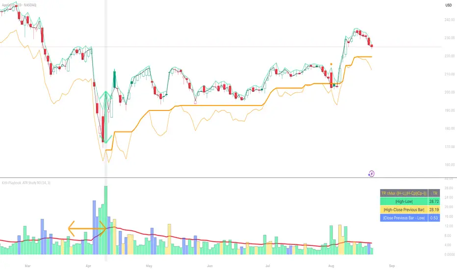
Kitti-Playbook ATR Study R0
Date : Aug 22 2025
Kitti-Playbook ATR Study R0
This is used to study the operation of the ATR Trailing Stop on the Long side, starting from the calculation of True Range.
1) Studying True Range Calculation
1.1) Specify the Bar graph you want to analyze for True Range.
Enable "Show Selected Price Bar" to locate the desired bar.
1.2) Enable/disable "Display True Range" in the Settings.
True Range is calculated as:
TR = Max (|H - L|, |H - Cp|, |Cp - L|)
• Show True Range:
Each color on the bar represents the maximum range value selected:
◦ |H - L| = Green
◦ |H - Cp| = Yellow
◦ |Cp - L| = Blue
• Show True Range on Selected Price Bar:
An arrow points to the range, and its color represents the maximum value chosen:
◦ |H - L| = Green
◦ |H - Cp| = Yellow
◦ |Cp - L| = Blue
• Show True Range Information Table:
Displays the actual values of |H - L|, |H - Cp|, and |Cp - L| from the selected bar.
2) Studying Average True Range (ATR)
2.1) Set the ATR Length in Settings.
Default value: ATR Length = 14
2.2) Enable/disable "Display Average True Range (RMA)" in Settings:
• Show ATR
• Show ATR Length from Selected Price Bar
(An arrow will point backward equal to the ATR Length)
3) Studying ATR Trailing
3.1) Set the ATR Multiplier in Settings.
Default value: ATR Multiply = 3
3.2) Enable/disable "Display ATR Trailing" in Settings:
• Show High Line
• Show ATR Bands
• Show ATR Trailing
4) Studying ATR Trailing Exit
(Occurs when the Close price crosses below the ATR Trailing line)
Enable/disable "Display ATR Trailing" in Settings:
• Show Close Line
• Show Exit Points
(Exit points are marked by an orange diamond symbol above the price bar)
Markov Chain [3D] | FractalystWhat exactly is a Markov Chain?
This indicator uses a Markov Chain model to analyze, quantify, and visualize the transitions between market regimes (Bull, Bear, Neutral) on your chart. It dynamically detects these regimes in real-time, calculates transition probabilities, and displays them as animated 3D spheres and arrows, giving traders intuitive insight into current and future market conditions.
How does a Markov Chain work, and how should I read this spheres-and-arrows diagram?
Think of three weather modes: Sunny, Rainy, Cloudy.
Each sphere is one mode. The loop on a sphere means “stay the same next step” (e.g., Sunny again tomorrow).
The arrows leaving a sphere show where things usually go next if they change (e.g., Sunny moving to Cloudy).
Some paths matter more than others. A more prominent loop means the current mode tends to persist. A more prominent outgoing arrow means a change to that destination is the usual next step.
Direction isn’t symmetric: moving Sunny→Cloudy can behave differently than Cloudy→Sunny.
Now relabel the spheres to markets: Bull, Bear, Neutral.
Spheres: market regimes (uptrend, downtrend, range).
Self‑loop: tendency for the current regime to continue on the next bar.
Arrows: the most common next regime if a switch happens.
How to read: Start at the sphere that matches current bar state. If the loop stands out, expect continuation. If one outgoing path stands out, that switch is the typical next step. Opposite directions can differ (Bear→Neutral doesn’t have to match Neutral→Bear).
What states and transitions are shown?
The three market states visualized are:
Bullish (Bull): Upward or strong-market regime.
Bearish (Bear): Downward or weak-market regime.
Neutral: Sideways or range-bound regime.
Bidirectional animated arrows and probability labels show how likely the market is to move from one regime to another (e.g., Bull → Bear or Neutral → Bull).
How does the regime detection system work?
You can use either built-in price returns (based on adaptive Z-score normalization) or supply three custom indicators (such as volume, oscillators, etc.).
Values are statistically normalized (Z-scored) over a configurable lookback period.
The normalized outputs are classified into Bull, Bear, or Neutral zones.
If using three indicators, their regime signals are averaged and smoothed for robustness.
How are transition probabilities calculated?
On every confirmed bar, the algorithm tracks the sequence of detected market states, then builds a rolling window of transitions.
The code maintains a transition count matrix for all regime pairs (e.g., Bull → Bear).
Transition probabilities are extracted for each possible state change using Laplace smoothing for numerical stability, and frequently updated in real-time.
What is unique about the visualization?
3D animated spheres represent each regime and change visually when active.
Animated, bidirectional arrows reveal transition probabilities and allow you to see both dominant and less likely regime flows.
Particles (moving dots) animate along the arrows, enhancing the perception of regime flow direction and speed.
All elements dynamically update with each new price bar, providing a live market map in an intuitive, engaging format.
Can I use custom indicators for regime classification?
Yes! Enable the "Custom Indicators" switch and select any three chart series as inputs. These will be normalized and combined (each with equal weight), broadening the regime classification beyond just price-based movement.
What does the “Lookback Period” control?
Lookback Period (default: 100) sets how much historical data builds the probability matrix. Shorter periods adapt faster to regime changes but may be noisier. Longer periods are more stable but slower to adapt.
How is this different from a Hidden Markov Model (HMM)?
It sets the window for both regime detection and probability calculations. Lower values make the system more reactive, but potentially noisier. Higher values smooth estimates and make the system more robust.
How is this Markov Chain different from a Hidden Markov Model (HMM)?
Markov Chain (as here): All market regimes (Bull, Bear, Neutral) are directly observable on the chart. The transition matrix is built from actual detected regimes, keeping the model simple and interpretable.
Hidden Markov Model: The actual regimes are unobservable ("hidden") and must be inferred from market output or indicator "emissions" using statistical learning algorithms. HMMs are more complex, can capture more subtle structure, but are harder to visualize and require additional machine learning steps for training.
A standard Markov Chain models transitions between observable states using a simple transition matrix, while a Hidden Markov Model assumes the true states are hidden (latent) and must be inferred from observable “emissions” like price or volume data. In practical terms, a Markov Chain is transparent and easier to implement and interpret; an HMM is more expressive but requires statistical inference to estimate hidden states from data.
Markov Chain: states are observable; you directly count or estimate transition probabilities between visible states. This makes it simpler, faster, and easier to validate and tune.
HMM: states are hidden; you only observe emissions generated by those latent states. Learning involves machine learning/statistical algorithms (commonly Baum–Welch/EM for training and Viterbi for decoding) to infer both the transition dynamics and the most likely hidden state sequence from data.
How does the indicator avoid “repainting” or look-ahead bias?
All regime changes and matrix updates happen only on confirmed (closed) bars, so no future data is leaked, ensuring reliable real-time operation.
Are there practical tuning tips?
Tune the Lookback Period for your asset/timeframe: shorter for fast markets, longer for stability.
Use custom indicators if your asset has unique regime drivers.
Watch for rapid changes in transition probabilities as early warning of a possible regime shift.
Who is this indicator for?
Quants and quantitative researchers exploring probabilistic market modeling, especially those interested in regime-switching dynamics and Markov models.
Programmers and system developers who need a probabilistic regime filter for systematic and algorithmic backtesting:
The Markov Chain indicator is ideally suited for programmatic integration via its bias output (1 = Bull, 0 = Neutral, -1 = Bear).
Although the visualization is engaging, the core output is designed for automated, rules-based workflows—not for discretionary/manual trading decisions.
Developers can connect the indicator’s output directly to their Pine Script logic (using input.source()), allowing rapid and robust backtesting of regime-based strategies.
It acts as a plug-and-play regime filter: simply plug the bias output into your entry/exit logic, and you have a scientifically robust, probabilistically-derived signal for filtering, timing, position sizing, or risk regimes.
The MC's output is intentionally "trinary" (1/0/-1), focusing on clear regime states for unambiguous decision-making in code. If you require nuanced, multi-probability or soft-label state vectors, consider expanding the indicator or stacking it with a probability-weighted logic layer in your scripting.
Because it avoids subjectivity, this approach is optimal for systematic quants, algo developers building backtested, repeatable strategies based on probabilistic regime analysis.
What's the mathematical foundation behind this?
The mathematical foundation behind this Markov Chain indicator—and probabilistic regime detection in finance—draws from two principal models: the (standard) Markov Chain and the Hidden Markov Model (HMM).
How to use this indicator programmatically?
The Markov Chain indicator automatically exports a bias value (+1 for Bullish, -1 for Bearish, 0 for Neutral) as a plot visible in the Data Window. This allows you to integrate its regime signal into your own scripts and strategies for backtesting, automation, or live trading.
Step-by-Step Integration with Pine Script (input.source)
Add the Markov Chain indicator to your chart.
This must be done first, since your custom script will "pull" the bias signal from the indicator's plot.
In your strategy, create an input using input.source()
Example:
//@version=5
strategy("MC Bias Strategy Example")
mcBias = input.source(close, "MC Bias Source")
After saving, go to your script’s settings. For the “MC Bias Source” input, select the plot/output of the Markov Chain indicator (typically its bias plot).
Use the bias in your trading logic
Example (long only on Bull, flat otherwise):
if mcBias == 1
strategy.entry("Long", strategy.long)
else
strategy.close("Long")
For more advanced workflows, combine mcBias with additional filters or trailing stops.
How does this work behind-the-scenes?
TradingView’s input.source() lets you use any plot from another indicator as a real-time, “live” data feed in your own script (source).
The selected bias signal is available to your Pine code as a variable, enabling logical decisions based on regime (trend-following, mean-reversion, etc.).
This enables powerful strategy modularity : decouple regime detection from entry/exit logic, allowing fast experimentation without rewriting core signal code.
Integrating 45+ Indicators with Your Markov Chain — How & Why
The Enhanced Custom Indicators Export script exports a massive suite of over 45 technical indicators—ranging from classic momentum (RSI, MACD, Stochastic, etc.) to trend, volume, volatility, and oscillator tools—all pre-calculated, centered/scaled, and available as plots.
// Enhanced Custom Indicators Export - 45 Technical Indicators
// Comprehensive technical analysis suite for advanced market regime detection
//@version=6
indicator('Enhanced Custom Indicators Export | Fractalyst', shorttitle='Enhanced CI Export', overlay=false, scale=scale.right, max_labels_count=500, max_lines_count=500)
// |----- Input Parameters -----| //
momentum_group = "Momentum Indicators"
trend_group = "Trend Indicators"
volume_group = "Volume Indicators"
volatility_group = "Volatility Indicators"
oscillator_group = "Oscillator Indicators"
display_group = "Display Settings"
// Common lengths
length_14 = input.int(14, "Standard Length (14)", minval=1, maxval=100, group=momentum_group)
length_20 = input.int(20, "Medium Length (20)", minval=1, maxval=200, group=trend_group)
length_50 = input.int(50, "Long Length (50)", minval=1, maxval=200, group=trend_group)
// Display options
show_table = input.bool(true, "Show Values Table", group=display_group)
table_size = input.string("Small", "Table Size", options= , group=display_group)
// |----- MOMENTUM INDICATORS (15 indicators) -----| //
// 1. RSI (Relative Strength Index)
rsi_14 = ta.rsi(close, length_14)
rsi_centered = rsi_14 - 50
// 2. Stochastic Oscillator
stoch_k = ta.stoch(close, high, low, length_14)
stoch_d = ta.sma(stoch_k, 3)
stoch_centered = stoch_k - 50
// 3. Williams %R
williams_r = ta.stoch(close, high, low, length_14) - 100
// 4. MACD (Moving Average Convergence Divergence)
= ta.macd(close, 12, 26, 9)
// 5. Momentum (Rate of Change)
momentum = ta.mom(close, length_14)
momentum_pct = (momentum / close ) * 100
// 6. Rate of Change (ROC)
roc = ta.roc(close, length_14)
// 7. Commodity Channel Index (CCI)
cci = ta.cci(close, length_20)
// 8. Money Flow Index (MFI)
mfi = ta.mfi(close, length_14)
mfi_centered = mfi - 50
// 9. Awesome Oscillator (AO)
ao = ta.sma(hl2, 5) - ta.sma(hl2, 34)
// 10. Accelerator Oscillator (AC)
ac = ao - ta.sma(ao, 5)
// 11. Chande Momentum Oscillator (CMO)
cmo = ta.cmo(close, length_14)
// 12. Detrended Price Oscillator (DPO)
dpo = close - ta.sma(close, length_20)
// 13. Price Oscillator (PPO)
ppo = ta.sma(close, 12) - ta.sma(close, 26)
ppo_pct = (ppo / ta.sma(close, 26)) * 100
// 14. TRIX
trix_ema1 = ta.ema(close, length_14)
trix_ema2 = ta.ema(trix_ema1, length_14)
trix_ema3 = ta.ema(trix_ema2, length_14)
trix = ta.roc(trix_ema3, 1) * 10000
// 15. Klinger Oscillator
klinger = ta.ema(volume * (high + low + close) / 3, 34) - ta.ema(volume * (high + low + close) / 3, 55)
// 16. Fisher Transform
fisher_hl2 = 0.5 * (hl2 - ta.lowest(hl2, 10)) / (ta.highest(hl2, 10) - ta.lowest(hl2, 10)) - 0.25
fisher = 0.5 * math.log((1 + fisher_hl2) / (1 - fisher_hl2))
// 17. Stochastic RSI
stoch_rsi = ta.stoch(rsi_14, rsi_14, rsi_14, length_14)
stoch_rsi_centered = stoch_rsi - 50
// 18. Relative Vigor Index (RVI)
rvi_num = ta.swma(close - open)
rvi_den = ta.swma(high - low)
rvi = rvi_den != 0 ? rvi_num / rvi_den : 0
// 19. Balance of Power (BOP)
bop = (close - open) / (high - low)
// |----- TREND INDICATORS (10 indicators) -----| //
// 20. Simple Moving Average Momentum
sma_20 = ta.sma(close, length_20)
sma_momentum = ((close - sma_20) / sma_20) * 100
// 21. Exponential Moving Average Momentum
ema_20 = ta.ema(close, length_20)
ema_momentum = ((close - ema_20) / ema_20) * 100
// 22. Parabolic SAR
sar = ta.sar(0.02, 0.02, 0.2)
sar_trend = close > sar ? 1 : -1
// 23. Linear Regression Slope
lr_slope = ta.linreg(close, length_20, 0) - ta.linreg(close, length_20, 1)
// 24. Moving Average Convergence (MAC)
mac = ta.sma(close, 10) - ta.sma(close, 30)
// 25. Trend Intensity Index (TII)
tii_sum = 0.0
for i = 1 to length_20
tii_sum += close > close ? 1 : 0
tii = (tii_sum / length_20) * 100
// 26. Ichimoku Cloud Components
ichimoku_tenkan = (ta.highest(high, 9) + ta.lowest(low, 9)) / 2
ichimoku_kijun = (ta.highest(high, 26) + ta.lowest(low, 26)) / 2
ichimoku_signal = ichimoku_tenkan > ichimoku_kijun ? 1 : -1
// 27. MESA Adaptive Moving Average (MAMA)
mama_alpha = 2.0 / (length_20 + 1)
mama = ta.ema(close, length_20)
mama_momentum = ((close - mama) / mama) * 100
// 28. Zero Lag Exponential Moving Average (ZLEMA)
zlema_lag = math.round((length_20 - 1) / 2)
zlema_data = close + (close - close )
zlema = ta.ema(zlema_data, length_20)
zlema_momentum = ((close - zlema) / zlema) * 100
// |----- VOLUME INDICATORS (6 indicators) -----| //
// 29. On-Balance Volume (OBV)
obv = ta.obv
// 30. Volume Rate of Change (VROC)
vroc = ta.roc(volume, length_14)
// 31. Price Volume Trend (PVT)
pvt = ta.pvt
// 32. Negative Volume Index (NVI)
nvi = 0.0
nvi := volume < volume ? nvi + ((close - close ) / close ) * nvi : nvi
// 33. Positive Volume Index (PVI)
pvi = 0.0
pvi := volume > volume ? pvi + ((close - close ) / close ) * pvi : pvi
// 34. Volume Oscillator
vol_osc = ta.sma(volume, 5) - ta.sma(volume, 10)
// 35. Ease of Movement (EOM)
eom_distance = high - low
eom_box_height = volume / 1000000
eom = eom_box_height != 0 ? eom_distance / eom_box_height : 0
eom_sma = ta.sma(eom, length_14)
// 36. Force Index
force_index = volume * (close - close )
force_index_sma = ta.sma(force_index, length_14)
// |----- VOLATILITY INDICATORS (10 indicators) -----| //
// 37. Average True Range (ATR)
atr = ta.atr(length_14)
atr_pct = (atr / close) * 100
// 38. Bollinger Bands Position
bb_basis = ta.sma(close, length_20)
bb_dev = 2.0 * ta.stdev(close, length_20)
bb_upper = bb_basis + bb_dev
bb_lower = bb_basis - bb_dev
bb_position = bb_dev != 0 ? (close - bb_basis) / bb_dev : 0
bb_width = bb_dev != 0 ? (bb_upper - bb_lower) / bb_basis * 100 : 0
// 39. Keltner Channels Position
kc_basis = ta.ema(close, length_20)
kc_range = ta.ema(ta.tr, length_20)
kc_upper = kc_basis + (2.0 * kc_range)
kc_lower = kc_basis - (2.0 * kc_range)
kc_position = kc_range != 0 ? (close - kc_basis) / kc_range : 0
// 40. Donchian Channels Position
dc_upper = ta.highest(high, length_20)
dc_lower = ta.lowest(low, length_20)
dc_basis = (dc_upper + dc_lower) / 2
dc_position = (dc_upper - dc_lower) != 0 ? (close - dc_basis) / (dc_upper - dc_lower) : 0
// 41. Standard Deviation
std_dev = ta.stdev(close, length_20)
std_dev_pct = (std_dev / close) * 100
// 42. Relative Volatility Index (RVI)
rvi_up = ta.stdev(close > close ? close : 0, length_14)
rvi_down = ta.stdev(close < close ? close : 0, length_14)
rvi_total = rvi_up + rvi_down
rvi_volatility = rvi_total != 0 ? (rvi_up / rvi_total) * 100 : 50
// 43. Historical Volatility
hv_returns = math.log(close / close )
hv = ta.stdev(hv_returns, length_20) * math.sqrt(252) * 100
// 44. Garman-Klass Volatility
gk_vol = math.log(high/low) * math.log(high/low) - (2*math.log(2)-1) * math.log(close/open) * math.log(close/open)
gk_volatility = math.sqrt(ta.sma(gk_vol, length_20)) * 100
// 45. Parkinson Volatility
park_vol = math.log(high/low) * math.log(high/low)
parkinson = math.sqrt(ta.sma(park_vol, length_20) / (4 * math.log(2))) * 100
// 46. Rogers-Satchell Volatility
rs_vol = math.log(high/close) * math.log(high/open) + math.log(low/close) * math.log(low/open)
rogers_satchell = math.sqrt(ta.sma(rs_vol, length_20)) * 100
// |----- OSCILLATOR INDICATORS (5 indicators) -----| //
// 47. Elder Ray Index
elder_bull = high - ta.ema(close, 13)
elder_bear = low - ta.ema(close, 13)
elder_power = elder_bull + elder_bear
// 48. Schaff Trend Cycle (STC)
stc_macd = ta.ema(close, 23) - ta.ema(close, 50)
stc_k = ta.stoch(stc_macd, stc_macd, stc_macd, 10)
stc_d = ta.ema(stc_k, 3)
stc = ta.stoch(stc_d, stc_d, stc_d, 10)
// 49. Coppock Curve
coppock_roc1 = ta.roc(close, 14)
coppock_roc2 = ta.roc(close, 11)
coppock = ta.wma(coppock_roc1 + coppock_roc2, 10)
// 50. Know Sure Thing (KST)
kst_roc1 = ta.roc(close, 10)
kst_roc2 = ta.roc(close, 15)
kst_roc3 = ta.roc(close, 20)
kst_roc4 = ta.roc(close, 30)
kst = ta.sma(kst_roc1, 10) + 2*ta.sma(kst_roc2, 10) + 3*ta.sma(kst_roc3, 10) + 4*ta.sma(kst_roc4, 15)
// 51. Percentage Price Oscillator (PPO)
ppo_line = ((ta.ema(close, 12) - ta.ema(close, 26)) / ta.ema(close, 26)) * 100
ppo_signal = ta.ema(ppo_line, 9)
ppo_histogram = ppo_line - ppo_signal
// |----- PLOT MAIN INDICATORS -----| //
// Plot key momentum indicators
plot(rsi_centered, title="01_RSI_Centered", color=color.purple, linewidth=1)
plot(stoch_centered, title="02_Stoch_Centered", color=color.blue, linewidth=1)
plot(williams_r, title="03_Williams_R", color=color.red, linewidth=1)
plot(macd_histogram, title="04_MACD_Histogram", color=color.orange, linewidth=1)
plot(cci, title="05_CCI", color=color.green, linewidth=1)
// Plot trend indicators
plot(sma_momentum, title="06_SMA_Momentum", color=color.navy, linewidth=1)
plot(ema_momentum, title="07_EMA_Momentum", color=color.maroon, linewidth=1)
plot(sar_trend, title="08_SAR_Trend", color=color.teal, linewidth=1)
plot(lr_slope, title="09_LR_Slope", color=color.lime, linewidth=1)
plot(mac, title="10_MAC", color=color.fuchsia, linewidth=1)
// Plot volatility indicators
plot(atr_pct, title="11_ATR_Pct", color=color.yellow, linewidth=1)
plot(bb_position, title="12_BB_Position", color=color.aqua, linewidth=1)
plot(kc_position, title="13_KC_Position", color=color.olive, linewidth=1)
plot(std_dev_pct, title="14_StdDev_Pct", color=color.silver, linewidth=1)
plot(bb_width, title="15_BB_Width", color=color.gray, linewidth=1)
// Plot volume indicators
plot(vroc, title="16_VROC", color=color.blue, linewidth=1)
plot(eom_sma, title="17_EOM", color=color.red, linewidth=1)
plot(vol_osc, title="18_Vol_Osc", color=color.green, linewidth=1)
plot(force_index_sma, title="19_Force_Index", color=color.orange, linewidth=1)
plot(obv, title="20_OBV", color=color.purple, linewidth=1)
// Plot additional oscillators
plot(ao, title="21_Awesome_Osc", color=color.navy, linewidth=1)
plot(cmo, title="22_CMO", color=color.maroon, linewidth=1)
plot(dpo, title="23_DPO", color=color.teal, linewidth=1)
plot(trix, title="24_TRIX", color=color.lime, linewidth=1)
plot(fisher, title="25_Fisher", color=color.fuchsia, linewidth=1)
// Plot more momentum indicators
plot(mfi_centered, title="26_MFI_Centered", color=color.yellow, linewidth=1)
plot(ac, title="27_AC", color=color.aqua, linewidth=1)
plot(ppo_pct, title="28_PPO_Pct", color=color.olive, linewidth=1)
plot(stoch_rsi_centered, title="29_StochRSI_Centered", color=color.silver, linewidth=1)
plot(klinger, title="30_Klinger", color=color.gray, linewidth=1)
// Plot trend continuation
plot(tii, title="31_TII", color=color.blue, linewidth=1)
plot(ichimoku_signal, title="32_Ichimoku_Signal", color=color.red, linewidth=1)
plot(mama_momentum, title="33_MAMA_Momentum", color=color.green, linewidth=1)
plot(zlema_momentum, title="34_ZLEMA_Momentum", color=color.orange, linewidth=1)
plot(bop, title="35_BOP", color=color.purple, linewidth=1)
// Plot volume continuation
plot(nvi, title="36_NVI", color=color.navy, linewidth=1)
plot(pvi, title="37_PVI", color=color.maroon, linewidth=1)
plot(momentum_pct, title="38_Momentum_Pct", color=color.teal, linewidth=1)
plot(roc, title="39_ROC", color=color.lime, linewidth=1)
plot(rvi, title="40_RVI", color=color.fuchsia, linewidth=1)
// Plot volatility continuation
plot(dc_position, title="41_DC_Position", color=color.yellow, linewidth=1)
plot(rvi_volatility, title="42_RVI_Volatility", color=color.aqua, linewidth=1)
plot(hv, title="43_Historical_Vol", color=color.olive, linewidth=1)
plot(gk_volatility, title="44_GK_Volatility", color=color.silver, linewidth=1)
plot(parkinson, title="45_Parkinson_Vol", color=color.gray, linewidth=1)
// Plot final oscillators
plot(rogers_satchell, title="46_RS_Volatility", color=color.blue, linewidth=1)
plot(elder_power, title="47_Elder_Power", color=color.red, linewidth=1)
plot(stc, title="48_STC", color=color.green, linewidth=1)
plot(coppock, title="49_Coppock", color=color.orange, linewidth=1)
plot(kst, title="50_KST", color=color.purple, linewidth=1)
// Plot final indicators
plot(ppo_histogram, title="51_PPO_Histogram", color=color.navy, linewidth=1)
plot(pvt, title="52_PVT", color=color.maroon, linewidth=1)
// |----- Reference Lines -----| //
hline(0, "Zero Line", color=color.gray, linestyle=hline.style_dashed, linewidth=1)
hline(50, "Midline", color=color.gray, linestyle=hline.style_dotted, linewidth=1)
hline(-50, "Lower Midline", color=color.gray, linestyle=hline.style_dotted, linewidth=1)
hline(25, "Upper Threshold", color=color.gray, linestyle=hline.style_dotted, linewidth=1)
hline(-25, "Lower Threshold", color=color.gray, linestyle=hline.style_dotted, linewidth=1)
// |----- Enhanced Information Table -----| //
if show_table and barstate.islast
table_position = position.top_right
table_text_size = table_size == "Tiny" ? size.tiny : table_size == "Small" ? size.small : size.normal
var table info_table = table.new(table_position, 3, 18, bgcolor=color.new(color.white, 85), border_width=1, border_color=color.gray)
// Headers
table.cell(info_table, 0, 0, 'Category', text_color=color.black, text_size=table_text_size, bgcolor=color.new(color.blue, 70))
table.cell(info_table, 1, 0, 'Indicator', text_color=color.black, text_size=table_text_size, bgcolor=color.new(color.blue, 70))
table.cell(info_table, 2, 0, 'Value', text_color=color.black, text_size=table_text_size, bgcolor=color.new(color.blue, 70))
// Key Momentum Indicators
table.cell(info_table, 0, 1, 'MOMENTUM', text_color=color.purple, text_size=table_text_size, bgcolor=color.new(color.purple, 90))
table.cell(info_table, 1, 1, 'RSI Centered', text_color=color.purple, text_size=table_text_size)
table.cell(info_table, 2, 1, str.tostring(rsi_centered, '0.00'), text_color=color.purple, text_size=table_text_size)
table.cell(info_table, 0, 2, '', text_color=color.blue, text_size=table_text_size)
table.cell(info_table, 1, 2, 'Stoch Centered', text_color=color.blue, text_size=table_text_size)
table.cell(info_table, 2, 2, str.tostring(stoch_centered, '0.00'), text_color=color.blue, text_size=table_text_size)
table.cell(info_table, 0, 3, '', text_color=color.red, text_size=table_text_size)
table.cell(info_table, 1, 3, 'Williams %R', text_color=color.red, text_size=table_text_size)
table.cell(info_table, 2, 3, str.tostring(williams_r, '0.00'), text_color=color.red, text_size=table_text_size)
table.cell(info_table, 0, 4, '', text_color=color.orange, text_size=table_text_size)
table.cell(info_table, 1, 4, 'MACD Histogram', text_color=color.orange, text_size=table_text_size)
table.cell(info_table, 2, 4, str.tostring(macd_histogram, '0.000'), text_color=color.orange, text_size=table_text_size)
table.cell(info_table, 0, 5, '', text_color=color.green, text_size=table_text_size)
table.cell(info_table, 1, 5, 'CCI', text_color=color.green, text_size=table_text_size)
table.cell(info_table, 2, 5, str.tostring(cci, '0.00'), text_color=color.green, text_size=table_text_size)
// Key Trend Indicators
table.cell(info_table, 0, 6, 'TREND', text_color=color.navy, text_size=table_text_size, bgcolor=color.new(color.navy, 90))
table.cell(info_table, 1, 6, 'SMA Momentum %', text_color=color.navy, text_size=table_text_size)
table.cell(info_table, 2, 6, str.tostring(sma_momentum, '0.00'), text_color=color.navy, text_size=table_text_size)
table.cell(info_table, 0, 7, '', text_color=color.maroon, text_size=table_text_size)
table.cell(info_table, 1, 7, 'EMA Momentum %', text_color=color.maroon, text_size=table_text_size)
table.cell(info_table, 2, 7, str.tostring(ema_momentum, '0.00'), text_color=color.maroon, text_size=table_text_size)
table.cell(info_table, 0, 8, '', text_color=color.teal, text_size=table_text_size)
table.cell(info_table, 1, 8, 'SAR Trend', text_color=color.teal, text_size=table_text_size)
table.cell(info_table, 2, 8, str.tostring(sar_trend, '0'), text_color=color.teal, text_size=table_text_size)
table.cell(info_table, 0, 9, '', text_color=color.lime, text_size=table_text_size)
table.cell(info_table, 1, 9, 'Linear Regression', text_color=color.lime, text_size=table_text_size)
table.cell(info_table, 2, 9, str.tostring(lr_slope, '0.000'), text_color=color.lime, text_size=table_text_size)
// Key Volatility Indicators
table.cell(info_table, 0, 10, 'VOLATILITY', text_color=color.yellow, text_size=table_text_size, bgcolor=color.new(color.yellow, 90))
table.cell(info_table, 1, 10, 'ATR %', text_color=color.yellow, text_size=table_text_size)
table.cell(info_table, 2, 10, str.tostring(atr_pct, '0.00'), text_color=color.yellow, text_size=table_text_size)
table.cell(info_table, 0, 11, '', text_color=color.aqua, text_size=table_text_size)
table.cell(info_table, 1, 11, 'BB Position', text_color=color.aqua, text_size=table_text_size)
table.cell(info_table, 2, 11, str.tostring(bb_position, '0.00'), text_color=color.aqua, text_size=table_text_size)
table.cell(info_table, 0, 12, '', text_color=color.olive, text_size=table_text_size)
table.cell(info_table, 1, 12, 'KC Position', text_color=color.olive, text_size=table_text_size)
table.cell(info_table, 2, 12, str.tostring(kc_position, '0.00'), text_color=color.olive, text_size=table_text_size)
// Key Volume Indicators
table.cell(info_table, 0, 13, 'VOLUME', text_color=color.blue, text_size=table_text_size, bgcolor=color.new(color.blue, 90))
table.cell(info_table, 1, 13, 'Volume ROC', text_color=color.blue, text_size=table_text_size)
table.cell(info_table, 2, 13, str.tostring(vroc, '0.00'), text_color=color.blue, text_size=table_text_size)
table.cell(info_table, 0, 14, '', text_color=color.red, text_size=table_text_size)
table.cell(info_table, 1, 14, 'EOM', text_color=color.red, text_size=table_text_size)
table.cell(info_table, 2, 14, str.tostring(eom_sma, '0.000'), text_color=color.red, text_size=table_text_size)
// Key Oscillators
table.cell(info_table, 0, 15, 'OSCILLATORS', text_color=color.purple, text_size=table_text_size, bgcolor=color.new(color.purple, 90))
table.cell(info_table, 1, 15, 'Awesome Osc', text_color=color.blue, text_size=table_text_size)
table.cell(info_table, 2, 15, str.tostring(ao, '0.000'), text_color=color.blue, text_size=table_text_size)
table.cell(info_table, 0, 16, '', text_color=color.red, text_size=table_text_size)
table.cell(info_table, 1, 16, 'Fisher Transform', text_color=color.red, text_size=table_text_size)
table.cell(info_table, 2, 16, str.tostring(fisher, '0.000'), text_color=color.red, text_size=table_text_size)
// Summary Statistics
table.cell(info_table, 0, 17, 'SUMMARY', text_color=color.black, text_size=table_text_size, bgcolor=color.new(color.gray, 70))
table.cell(info_table, 1, 17, 'Total Indicators: 52', text_color=color.black, text_size=table_text_size)
regime_color = rsi_centered > 10 ? color.green : rsi_centered < -10 ? color.red : color.gray
regime_text = rsi_centered > 10 ? "BULLISH" : rsi_centered < -10 ? "BEARISH" : "NEUTRAL"
table.cell(info_table, 2, 17, regime_text, text_color=regime_color, text_size=table_text_size)
This makes it the perfect “indicator backbone” for quantitative and systematic traders who want to prototype, combine, and test new regime detection models—especially in combination with the Markov Chain indicator.
How to use this script with the Markov Chain for research and backtesting:
Add the Enhanced Indicator Export to your chart.
Every calculated indicator is available as an individual data stream.
Connect the indicator(s) you want as custom input(s) to the Markov Chain’s “Custom Indicators” option.
In the Markov Chain indicator’s settings, turn ON the custom indicator mode.
For each of the three custom indicator inputs, select the exported plot from the Enhanced Export script—the menu lists all 45+ signals by name.
This creates a powerful, modular regime-detection engine where you can mix-and-match momentum, trend, volume, or custom combinations for advanced filtering.
Backtest regime logic directly.
Once you’ve connected your chosen indicators, the Markov Chain script performs regime detection (Bull/Neutral/Bear) based on your selected features—not just price returns.
The regime detection is robust, automatically normalized (using Z-score), and outputs bias (1, -1, 0) for plug-and-play integration.
Export the regime bias for programmatic use.
As described above, use input.source() in your Pine Script strategy or system and link the bias output.
You can now filter signals, control trade direction/size, or design pairs-trading that respect true, indicator-driven market regimes.
With this framework, you’re not limited to static or simplistic regime filters. You can rigorously define, test, and refine what “market regime” means for your strategies—using the technical features that matter most to you.
Optimize your signal generation by backtesting across a universe of meaningful indicator blends.
Enhance risk management with objective, real-time regime boundaries.
Accelerate your research: iterate quickly, swap indicator components, and see results with minimal code changes.
Automate multi-asset or pairs-trading by integrating regime context directly into strategy logic.
Add both scripts to your chart, connect your preferred features, and start investigating your best regime-based trades—entirely within the TradingView ecosystem.
References & Further Reading
Ang, A., & Bekaert, G. (2002). “Regime Switches in Interest Rates.” Journal of Business & Economic Statistics, 20(2), 163–182.
Hamilton, J. D. (1989). “A New Approach to the Economic Analysis of Nonstationary Time Series and the Business Cycle.” Econometrica, 57(2), 357–384.
Markov, A. A. (1906). "Extension of the Limit Theorems of Probability Theory to a Sum of Variables Connected in a Chain." The Notes of the Imperial Academy of Sciences of St. Petersburg.
Guidolin, M., & Timmermann, A. (2007). “Asset Allocation under Multivariate Regime Switching.” Journal of Economic Dynamics and Control, 31(11), 3503–3544.
Murphy, J. J. (1999). Technical Analysis of the Financial Markets. New York Institute of Finance.
Brock, W., Lakonishok, J., & LeBaron, B. (1992). “Simple Technical Trading Rules and the Stochastic Properties of Stock Returns.” Journal of Finance, 47(5), 1731–1764.
Zucchini, W., MacDonald, I. L., & Langrock, R. (2017). Hidden Markov Models for Time Series: An Introduction Using R (2nd ed.). Chapman and Hall/CRC.
On Quantitative Finance and Markov Models:
Lo, A. W., & Hasanhodzic, J. (2009). The Heretics of Finance: Conversations with Leading Practitioners of Technical Analysis. Bloomberg Press.
Patterson, S. (2016). The Man Who Solved the Market: How Jim Simons Launched the Quant Revolution. Penguin Press.
TradingView Pine Script Documentation: www.tradingview.com
TradingView Blog: “Use an Input From Another Indicator With Your Strategy” www.tradingview.com
GeeksforGeeks: “What is the Difference Between Markov Chains and Hidden Markov Models?” www.geeksforgeeks.org
What makes this indicator original and unique?
- On‑chart, real‑time Markov. The chain is drawn directly on your chart. You see the current regime, its tendency to stay (self‑loop), and the usual next step (arrows) as bars confirm.
- Source‑agnostic by design. The engine runs on any series you select via input.source() — price, your own oscillator, a composite score, anything you compute in the script.
- Automatic normalization + regime mapping. Different inputs live on different scales. The script standardizes your chosen source and maps it into clear regimes (e.g., Bull / Bear / Neutral) without you micromanaging thresholds each time.
- Rolling, bar‑by‑bar learning. Transition tendencies are computed from a rolling window of confirmed bars. What you see is exactly what the market did in that window.
- Fast experimentation. Switch the source, adjust the window, and the Markov view updates instantly. It’s a rapid way to test ideas and feel regime persistence/switch behavior.
Integrate your own signals (using input.source())
- In settings, choose the Source . This is powered by input.source() .
- Feed it price, an indicator you compute inside the script, or a custom composite series.
- The script will automatically normalize that series and process it through the Markov engine, mapping it to regimes and updating the on‑chart spheres/arrows in real time.
Credits:
Deep gratitude to @RicardoSantos for both the foundational Markov chain processing engine and inspiring open-source contributions, which made advanced probabilistic market modeling accessible to the TradingView community.
Special thanks to @Alien_Algorithms for the innovative and visually stunning 3D sphere logic that powers the indicator’s animated, regime-based visualization.
Disclaimer
This tool summarizes recent behavior. It is not financial advice and not a guarantee of future results.

Parabolic Stoch SAR VisualizerParabolic Stoch SAR Visualizer — Momentum-Driven Trend Precision Tool
Overview:
Parabolic Stoch SAR Visualizer is a thoughtfully engineered hybrid indicator that blends momentum oscillation and trend-following mechanics into one robust system. By applying a custom Parabolic SAR calculation directly on a double-smoothed stochastic oscillator (rather than on price), it generates cleaner signals with enhanced trend detection and fewer false positives than typical Parabolic RSI or standard SAR variants.
Unique Functionality:
Momentum smoothing : The base stochastic %K undergoes double smoothing via consecutive simple moving averages, significantly cutting down random noise and erratic swings common in raw stochastic readings. This stabilizes momentum tracking, isolating true price strength and weakness.
Custom Parabolic SAR on smoothed momentum : Traditional SAR algorithms operate on price data, acting as trailing stops. This indicator repurposes SAR to work on smoothed stochastic values, effectively converting it into a momentum-driven directional filter. This yields a more adaptive and responsive trend signal focused on genuine momentum shifts instead of price noise.
Bounded SAR range and adjustable acceleration : SAR values are mathematically restricted between 0 and 100, aligning with the stochastic scale to prevent distortions. Traders can customize acceleration parameters (start, increment, max) to fine-tune trend sensitivity relative to market volatility or specific strategies.
Signal clarity through filterin g: Minimum bar spacing and minimum SAR movement thresholds between plotted dots reduce chart clutter, highlighting only meaningful trend changes and filtering out insignificant fluctuations.
Enhanced visuals : The oscillator line smoothly transitions its color gradient between defined uptrend and downtrend hues, intuitively signaling momentum strength. Parabolic SAR dots are offset from the oscillator line with multi-layered glow effects, making trend flips easy to spot at a glance.
Trading Application:
Trend identification : Momentum-based SAR dots offer precise marking of trend shifts, helping traders avoid false breakouts and premature trades.
Entry and exit timing : Combining the double-smoothed stochastic oscillator and SAR dots creates a reliable framework to confirm momentum shifts and optimal trade entries or exits.
Customizable for volatility regimes : Adjustable acceleration and filtering parameters allow scalpers to increase signal sensitivity, while swing traders can dial back noise for smoother trend recognition.
Visual clarity for fast decisions : Gradient color coding and glowing SAR dots facilitate immediate momentum assessment without complex analysis, empowering quicker, more confident trade actions.
Advantages over Parabolic RSI and similar indicators:
Parabolic RSI’s direct application of SAR on RSI often results in noisy, choppy signals prone to whipsaws. This indicator’s double-smoothed stochastic foundation delivers a cleaner, steadier signal.
Applying SAR to smoothed momentum rather than price transforms it into a directional filter that better captures true market strength with reduced lag.
Adaptive plotting thresholds and enhanced visuals minimize clutter and ambiguity, improving trader focus and execution speed.

Smart Impulse Exhaustion Finder (ATR + ADX Filter)📌 Purpose
This indicator detects potential exhaustion of strong bullish or bearish impulses at fresh swing highs/lows by combining multiple price action and volatility-based filters.
🧠 How It Works
A signal is triggered only when all core conditions are satisfied:
1. Swing High/Low Detection
Current high (or low) must be the highest (or lowest) over the last Extremum Lookback bars (default: 50).
This ensures the move is significant relative to recent price action.
2. Impulse Confirmation
Price must extend by at least 1 × ATR from the previous swing point.
This filters out minor fluctuations.
3. Exhaustion Conditions (at least 2 out of 3 must be met)
RSI Extreme: RSI > Overbought Level (default: 80) for bearish signals, RSI < Oversold Level (default: 20) for bullish signals.
Volume Spike: Volume > SMA(Volume, Volume SMA Length) × Volume Spike Multiplier.
Candle Wick Rejection: Upper wick ≥ Wick Threshold % for bearish setups, Lower wick ≥ Wick Threshold % for bullish setups.
4. Trend Filter
ADX > ADX Threshold ensures the market is trending and filters out sideways conditions.
5. Candle Body Filter
Candle body must be ≥ Body Size ATR Factor × ATR.
This avoids weak signals from small candles or doji formations.
📈 How to Use
Bearish Signal:
Appears at fresh swing highs with exhaustion conditions met. Useful for tightening stops, taking partial profits, or counter-trend shorts.
Bullish Signal:
Appears at fresh swing lows with exhaustion conditions met. Useful for trailing stops, profit-taking, or counter-trend longs.
Recommended Timeframes: Works best on 1h, 4h, and Daily charts.
Markets: Crypto, Forex, Stocks — wherever volatility and trends are present.
⚙️ Inputs
RSI Length / Overbought / Oversold
Volume SMA Length & Volume Spike Multiplier
Wick Threshold %
Extremum Lookback (bars for highs/lows)
ADX Length & Threshold
Body Size ATR Factor
⚠️ Disclaimer
This script is for educational purposes only and does not constitute financial advice.
Always test thoroughly and apply proper risk management before live trading.
💡 Tip: Combine this tool with your own market context and confluence factors for higher probability setups.
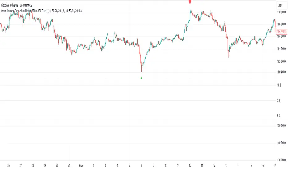
Price Exhaustion Envelope [BackQuant]Price Exhaustion Envelope
Visual preview of the bands:
What it is
The Price Exhaustion Envelope (PEE) is a multi‑factor overextension detector wrapped inside a dynamic envelope framework. It measures how “tired” a move is by blending price stretch, volume surges, momentum and acceleration, plus optional RSI divergence. The result is a composite exhaustion score that drives both on‑chart signals and the adaptive width of three optional envelope bands around a smoothed baseline. When the score spikes above or below your chosen threshold, the script can flag exhaustion, paint candles, tint the background and fire alerts.
How it works under the hood
Exhaustion score
Price component: distance of close from its mean in standard deviation units.
Volume component: normalized volume pressure that highlights unusual participation.
Momentum component: rate of change and acceleration of price, scaled by their own volatility.
RSI divergence (optional): bullish and bearish divergences gently push the score lower or higher.
Mode control: choose Price, Volume, Momentum or Composite. Composite averages the main pieces for a balanced view.
Energy scale (0 to 100)
The composite score is pushed through a logistic transform to create an “energy” value. High energy (above 70 to 80) signals a move that may be running hot, while very low energy (below 20 to 30) points to exhaustion on the downside.
Envelope engine
Baseline: EMA of price over the main lookback length.
Width: base width is standard deviation times a multiplier.
Type selector:
• Static keeps the width fixed.
• Dynamic expands width in proportion to the absolute exhaustion score.
• Adaptive links width to the energy reading so bands breathe with market “heat.”
Smoothing: a short EMA on the width reduces jitter and keeps bands pleasant to trade around.
Band architecture
You can toggle up to three symmetric bands on each side of the baseline. They default to 1.0, 1.6 and 2.2 multiples of the smoothed width. Soft transparent fills create a layered thermograph of extension. The outermost band often maps to true blow‑off extremes.
On‑chart elements
Baseline line that flips color in real time depending on where price sits.
Up to three upper and lower bands with progressive opacity.
Triangle markers at fresh exhaustion triggers.
Tiny warning glyphs at extreme upper or lower breaches.
Optional bar coloring to visually tag exhausted candles.
Background halo when energy > 80 or < 20 for instant context.
A compact info table showing State, Score, Energy, Momentum score and where price sits inside the envelope (percent).
How to use it in trading
Mean reversion plays
When price pierces the outer band and an exhaustion marker prints, look for reversal candles or lower‑timeframe confirmation to fade the move back toward the baseline.
For conservative entries, wait for the composite score to roll back under the threshold or for energy to drop from extreme to neutral.
Set stops just beyond the extreme levels (use extreme_upper and extreme_lower as natural invalidation points). Targets can be the baseline or the opposite inner band.
Trend continuation with smart pullbacks
In strong trends, the first tag of Band 1 or Band 2 against the dominant direction often offers low‑risk continuation entries. Use energy readings: if energy is low on a pullback during an uptrend, a bounce is more likely.
Combine with RSI divergence: hidden bullish divergence near a lower band in an uptrend can be a powerful confirmation.
Breakout filtering
A breakout that occurs while the composite score is still moderate (not exhausted) has a higher chance of follow‑through. Skip signals when energy is already above 80 and price is punching the outer band, as the move may be late.
Watch env_position (Envelope %) in the table. Breakouts near 40 to 60 percent of the envelope are “healthy,” while those at 95 percent are stretched.
Scaling out and risk control
Use exhaustion alerts to trim positions into strength or weakness.
Trail stops just outside Band 2 or Band 3 to stay in trends while letting the envelope expand in volatile phases.
Multi‑timeframe confluence
Run the script on a higher timeframe to locate exhaustion context, then drill down to a lower timeframe for entries.
Opposite signals across timeframes (daily exhaustion vs. 5‑minute breakout) warn you to reduce size or tighten management.
Key inputs to experiment with
Lookback Period: larger values smooth the score and envelope, ideal for swing trading. Shorter values make it reactive for scalps.
Exhaustion Threshold: raise above 2.0 in choppy assets to cut noise, drop to 1.5 for smooth FX pairs.
Envelope Type: Dynamic is great for crypto spikes, Adaptive shines in stocks where volume and volatility wave together.
RSI Divergence: turn off if you prefer a pure price/volume model or if divergence floods the score in your asset.
Alert set included
Fresh upper exhaustion
Fresh lower exhaustion
Extreme upper breach
Extreme lower breach
RSI bearish divergence
RSI bullish divergence
Hook these to TradingView notifications so you get pinged the moment a move hits exhaustion.
Best practices
Always pair exhaustion signals with structure. Support and resistance, liquidity pools and session opens matter.
Avoid blindly shorting every upper signal in a roaring bull market. Let the envelope type help you filter.
Use the table to sanity‑check: a very high score but mid‑range env_position means the band may still be wide enough to absorb more movement.
Backtest threshold combinations on your instrument. Different tickers carry different volatility fingerprints.
Final note
Price Exhaustion Envelope is a flexible framework, not a turnkey system. It excels as a context layer that tells you when the crowd is pressing too hard or when a move still has fuel. Combine it with sound execution tactics, risk limits and market awareness. Trade safe and let the envelope breathe with the market.
